Readings on Randomness -- Entropy

Entropy

The word entropy is used in several different ways in English, but it always refers to some notion of randomness, disorder, or uncertainty. For example, in physics the term is a measure of a system’s thermal energy, which is related to the level of random motion of molecules and hence is a measure of disorder. In general English usage, entropy is used as a less precise term but still refers to disorder or randomness. In settings that deal with computer and communication systems, entropy refers to its meaning in the field of information theory, where entropy has a very precise mathematical definition measuring randomness and uncertainty. Information theory grew out of the initial work of Claude Shannon at Bell Labs in the 1940’s, where he also did some significant work on the science of cryptography. The fundamental question of how information is represented is a common and deep thread connecting issues of communication, data compression, and cryptography, and information theory is a key component of all three of these areas. In honor of his work, this use of “entropy” is sometimes called “Shannon entropy.”

Entropy - Basic Model and Some Intuition

To talk precisely about the information content in messages, we first need a mathematical model that describes how information is transmitted. We consider an information source as having access to a set of possible messages, from which it selects a message, encodes it somehow, and transmits it across a communication channel.

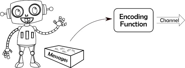
The question of encoding is very involved, and we can encode for the most compact representation (data compression), for the most reliable transmission (error detection/correction coding), to make the information unintelligible to an eavesdropper (encryption), or perhaps with other goals in mind. For now we focus just on how messages are selected, not how they are encoded.

How are messages selected? We take the source to be probabilistic. We’re not saying that data is really just randomly chosen, but this is a good model that has proved its usefulness over time.

Definition: A source is an ordered pair \({\cal S}=(M,P)\), where \(M=\{m_1,m_2,\cdots,m_n\}\) is a finite set, called the message space (or sometimes the source alphabet), and \(P:M\rightarrow [0,1]\) is a probability distribution on \(M\). We refer to the elements of \(M\) as messages. We denote the probability of message \(m_i\) by either \(P(m_i)\) or by the shorthand notation \(p_i\).

Intuitively, the higher the probability of a message, the lower the information content of that message. As an extreme example, if we knew in advance the message that was going to be sent (so the probability of that message is 1), then there is no information at all in that message – the receiver hasn’t learned anything new, since the message was pre-determined. Extending the idea of information from a single message to a source with multiple possible messages, a source with a large message space of small probability messages will have a higher information content than a source with a small message space or a few high probability messages.

Notice that when we are discussing information content of a source, we refer to the probabilities and the size of the message space. The actual messages do not matter, so “information” in this sense is different from using “information” to refer to semantic content of the messages. We can consider a function \(H\) that maps sources into information measures, and we use the notation \(H({\mathcal S})\) to denote information, or entropy, of a source. Since this measure only depends on the probability distribution, and not the message space, we sometimes just write \(H(P)\) for the entropy of a probability distribution. Alternatively, we can actually list the probabilities, and write this as \(H(p_1,p_2,\cdots,p_n)\). Next, we will see that the actual entropy function can be one of infinitely many choices, but the difference between the choices really just amounts to selecting different units of measurement (i.e., different scales).

Properties and Formal Definition

Using some intuition about the information content of a source, we can define several properties that a sensible information measure must obey.

Property 1. \(H\) is continuous for all valid probability distributions.

Property 2. For uniform probability spaces, the entropy of a source increases as the number of items in the message space increases. In other words, if \(U_n\) represents the uniform probability distribution on \(n\) items (so each has probability \(1/n\)), then \(H(U_n)<H(U_{n+1})\).

Property 3. If a message is picked in stages, then the information of the message is the sum of the information of the individual choices, weighted by the probability that that choice has to be made. For example, if we pick a playing card, the information content is the same whether we pick from the full set of 52 cards, or if we first pick the card color (red or black) and then pick the specific card from the chosen smaller set. Mathematically, this means that if our message space is made up of elements \(x_1,x_2,\cdots,x_n\) and \(y_1,y_2,\cdots,y_m\), with probabilities \(p_1,p_2,\cdots,p_n\) and \(q_1,q_2,\cdots,q_m\), respectively, and \(p=p_1+\cdots+p_n\) and \(q=q_1+\cdots+q_m\), then the entropy must satisfy

\[H(p_1,\cdots,p_n,q_1,\cdots,q_m) = H(p,q) + p H(\frac{p_1}{p},\frac{p_2}{p},\cdots,\frac{p_n}{p}) + q H(\frac{q_1}{q},\frac{q_2}{q},\cdots,\frac{q_m}{q}) .\]

Going back to our example with playing cards, we could let \(x_1,\cdots,x_n\) denote the red cards, and \(y_1,\cdots,y_m\) denote the black cards. Then \(H(p,q)\) represents the information content of selecting the card color (with probability \(p\) of picking red, and \(q\) of picking black), and then we select from either the red cards or the black cards.

Properties 1 and 2 are satisfied by many functions, but the following Theorem shows that property 3 is very restrictive. In fact, there is essentially only one function (ignoring constant factors) that satisfies all three properties.

Theorem: The only functions that satisfy properties 1-3 above are of the following form, where \({\mathcal S}=(M,P)\) is a source: \[H_b({\mathcal S}) = -\sum_{m\in M} P(m)\log_b P(m) = \sum_{m\in M} P(m)\log_b \frac{1}{P(m)} , \] for some constant \(b>0\).

This is actually a pretty amazing result: Given some very basic properties that any measure of information must satisfy, there is essentially just one function (up to constant factors) that we can use for such a measure! This pretty much removes all doubt about whether we have the “right measure” for entropy.

Given this result, and the natural use of base two logarithms in digital communication, we define entropy as follows.

Definition: The entropy of a source \({\cal S}=(S,P)\), denoted \(H({\cal S})\) or \(H(P)\), is defined by \[H({\mathcal S}) = -\sum_{m\in M} P(m)\log_2 P(m) = \sum_{m\in M} P(m)\log_2 \frac{1}{P(m)} , \] where the unit of information is a “bit.”

Example: Consider flipping a fair coin, where the messages represent heads and tails, each with probability 1/2. The entropy of this source is

\[ H\left(\frac{1}{2},\frac{1}{2}\right) = \frac{1}{2}\log_2 2 + \frac{1}{2}\log_2 2 = \frac{1}{2} + \frac{1}{2} = 1 . \]

In other words, the entropy of a source that flips a single fair coin is exactly 1 bit. This should match your basic notion of what a bit is: two outcomes, whether heads and tails, or true and false, or 0 and 1.

Example: We generalize the previous example to the uniform distribution on \(n\) outcomes, denoted \(U_n\), so each message has probability \(1/n\). In this case the entropy is

\[ H(U_n) = \sum_{i=1}^n \frac{1}{n}\log_2 n = n \cdot\frac{1}{n}\log_2 n = \log_2 n . \]

Applying this to rolling a fair 6-sided die, we see that the entropy of one roll is \(\log_2 6\approx 2.585\) bits.

If we pick a symmetric encryption key uniformly out of \(2^{128}\) possible keys, then the entropy of the key source is \(\log_2 2^{128}=128\) bits. Since this key is most likely just a randomly chosen 128-bit binary string, this makes sense.

Example: Consider picking a 128-bit random value, but instead of a uniform random number generator, we have a biased one in which each bit chosen with \(P(0)=1/10\) and \(P(1)=9/10\). We could use the binomial distribution to give the probability of any individual 128-bit string, but in this case we can take a much simpler shortcut: Using “Property 3” of the entropy function, we can analyze this as a sequence of 128 selections, and add the results up. In fact, since each selection (i.e., each bit) has the same probability distribution, independent of the others, the entropy of this source is just

\[ 128\cdot H\left(\frac{1}{10},\frac{9}{10}\right) = 128 \left( \frac{1}{10}\log_2\frac{10}{1} + \frac{9}{10}\log_2\frac{10}{9}\right) \approx 128\cdot 0.469 = 60.032 . \]

In other words, using a biased random number generator reduces the entropy of the source from 128 bits to around 60 bits. This can have serious consequences for security, which we’ll see below.

Entropy of English Language

One way we can view English language writing is as a sequence of individual letters, selected independently. Obviously this isn’t a great model of English, since letters in English writing aren’t independent, but this is a good starting point to think about the information content of English.

Many experiments by cryptographers and data compression researchers have shown that the frequency of individual letters is remarkably constant among different pieces of English writing. In one such study [J. Storer, Data Compression: Methods and Theory], the probability of a space is 0.1741, the probability of an ‘e’ is 0.0976, the probability of a ‘t’ is 0.0701, and so on. From these statistics, the entropy of English (from a source generating single letters) was calculated to be 4.47 bits.

We can make our model of English more accurate by considering pairs of letters rather than individual letters (what cryptographers call “digrams”). For example, the letter “q” is almost always followed by the letter “u” (the only exceptions being words derived from a foreign language, like “Iraqi,” “Iqbal,” and “Chongqing”). Therefore, the probability of the pair “qu” is much higher than would be expected when looking at letters independently, and hence the entropy is lower for modeling pairs of letters rather than individual letters. In the same experiment described in the previous paragraph, English was modeled as a source that produces pairs of letters, and the entropy of this source model was only 7.18 bits per pair of characters, or 3.59 bits per character.

We can go even farther by considering longer contexts when selecting the “next letter” in English. For example, if you see the letters “algori” then the next letter is almost certainly a “t”. What is the best model for a source generating English? Shannon had a great answer for this: The adult human mind has been trained for years to work with English, so he used an experiment with human subjects to estimate the entropy of English. In particular, he provided the subjects with a fragment of English text, and asked them to predict the next letter, and statistics were gathered on how often the subject guessed correctly. “Correct” versus “incorrect” doesn’t fully capture information content, but can provide bounds, and using this experiment Shannon estimated the “true entropy of English” to be between 0.6 and 1.3 bits per letter. Keep in mind that this was in the 1940’s, before Shannon had computers to help with the analysis. These days we have a huge amount of English text available for analysis by modern computers, and experiments that include the full ASCII character set (rather than just letters) consistently show that entropy of English writing is between 1.2 and 1.7 bits per character.

Passwords, Entropy, and Brute-Force Searches

This part is still being written!

Up: Contents Prev: Randomness Next: Pseudorandomness